Intro to Structured Prediction in 3 Acts

## Intro to Structured Prediction in 3 Acts Steve Ash [www.manycupsofcoffee.com](www.manycupsofcoffee.com)

### About Me * BA, MS, PhD (in Spring '17) Computer Science * 10 years building banking and healthcare software * 5 years leading a "skunkworks" R&D team

### Agenda * What is Structured Prediction? * **Act 1**: How to solve this problem in 1996? * _generative models_ * **Act 2**: How to solve this problem in 2006? * _discriminative models_ * **Act 3**: How to solve this problem in 2016? * _recurrent neural networks_

# Intro What is Structured Prediction?

### What is Structured Prediction Common machine learning tasks: * **Classification**: input data to fixed number of output classes/categories * Is this credit card transaction fraudulent? * Does this patient have liver disease? * **Regression**: input data to continuous output * Prospective student's future GPA based on information from his/her college application What about classification over a _sequence_ of information?

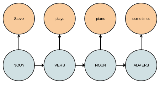
### What is Structured Prediction Assign part-of-speech tags to sequence of words: "Steve plays piano sometimes" ![Parts of Speech](/talks/pred-steve-pos-1.png)

### What is Structured Prediction The sequence of words — i.e. the _structure_ — affects the part-of-speech. We need to incorporate this structure into the predictive method that we want to use in order to improve our accuracy. Without the structure we can't disambiguate words that have more than one part-of-speech: > "Will Bob will the will to Will?"

### Quick background In probabilistic modeling we model our inputs and outputs as _random variables_. * Coin flip `$P(X=\textrm{heads})=0.5$` In the part-of-speech example, we had a sequence of words and a sequence of POS tags. * `$X_t$` = the word at time `$t$` * `$Y_t$` = the predicted POS tag at time `$t$` * `$P(Y_t=\textrm{NOUN}) = 0.1232$`

### Quick background Joint probability distribution `$$P(X=\textrm{will}, Y=\textrm{NOUN})$$` Conditional probability distribution `$$P(Y=\textrm{NOUN} | X=\textrm{will})$$` Relationship: `$P(X, Y)=P(X | Y) \times P(Y)$` Bayes Rule: `$P(Y | X)=\frac{P(X | Y) \times P(Y)}{P(X)}$`

Joint vs Conditional

Joint distribution knows everything about $P(X, Y)$

	NOUN	VERB	ADJ
dog	13423	34	0
walk	4300	7400	0
cat	12002	12	0
short	904	3123	4339

Frequency table- each cell is how many occurrences you have seen

Joint vs Conditional

Joint distribution knows everything about $P(X, Y)$

$P(X=\textrm{short}, Y=\textrm{VERB})=0.0686$

	NOUN	VERB	ADJ
dog	0.2948	0.0007	0.0000
walk	0.0944	0.1625	0.0000
cat	0.2636	0.0003	0.0000
short	0.0199	0.0686	0.0953

Joint distribution- each cell divided by sum of all counts

Joint vs Conditional

Conditional distribution only has information about a single row/column

$P(X=\textrm{short} | Y=\textrm{VERB}) = 0.2955$

	NOUN	VERB	ADJ
dog	0.2948	0.0007	0.0000
walk	0.0944	0.1625	0.0000
cat	0.2636	0.0003	0.0000
short	0.0199	0.0686	0.0953

	$P(X\|\textrm{VERB})$
dog	0.0032
walk	0.7002
cat	0.0011
short	0.2955

# Act 1 Generative Models

### Hidden Markov Models Assume that the thing you are interested in can be modeled as a sequence of **hidden** states, where at each state some value is **emitted**, and that's all you can see. Goal: find a **path** through the hidden states that best explains what you see States? paths? Sounds like a job for **automata** ![HMM states](/talks/pred-hmm-1.png)

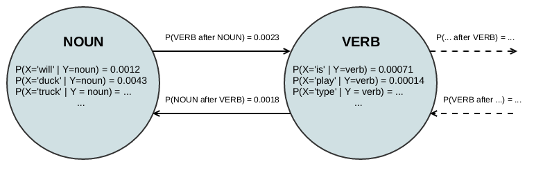
### Hidden Markov Models Models the real world process as: * Select a starting state (or have a single starting state) * **emit** an observed value from this state * **transition** to the next state * assume that you can predict the next state using only the previous $k$ states - **markov** property * ... | | `$t = 0$` | `$t = 1$` | `$t = 2$` | `$t = 3$` | |---------------|-----------|-----------|-----------|-----------| | Hidden State | NOUN | VERB | NOUN | ADVERB | | Emitted Value | Steve | plays | piano | sometimes |

### Hidden Markov Models Each path has an overall probability, and thus we want to find the most probable path.

* `$A_{ij}$` - prob of **transitioning** from state `$Y_i$` to `$Y_j$` * `$B_m(k)$` - prob of state $k$ **emitting** value $m$ * `$\pi_i$` - prob of **starting** from state $i$ `$\textbf{O}_t$` observed sequence: `$$\textbf{O}_0 = \textrm{Steve}, \textbf{O}_1 = \textrm{plays},\dots$$` `$\textbf{Q}_t$` hidden sequence: `$$\textbf{Q}_0 = \textrm{NOUN}, \textbf{Q}_1 = \textrm{VERB},\dots$$`

### Hidden Markov Models So our inference problem is: `$$P(Q | O) = \frac{P(O | Q) \times P(Q)}{P(O)}$$` Since the right hand numerator is `$P(O | Q) \times P(Q)$`, we basically have to estimate the whole joint probability distribution of words and POS tags. An interesting property of models formulated like this is that we can use the probability model to **generate** new instances from our data population.

### Hidden Markov Models Problems: * Each hidden state's emission probabilities is a probability distribution. * States with many possible emission values have to spread that probability mass out. * More states means lower and lower overall sequence probability * If we don't need to _generate_ values, we don't need the full joint distribution. We just want $P(Q | O)$...

# Act 2 Discriminative Models

### Conditional Random Fields In contrast to _generative_ models like HMMs, discriminative models don't bother trying to represent the real underlying process that results in the evidence that you observe. Instead they just model the output directly: `$P(Y | X)$` In 2001, a flexible, discriminative approach to structured prediction was introduced called: **Conditional Random Fields** (CRFs)

Conditional Random Fields

CRF Schematic

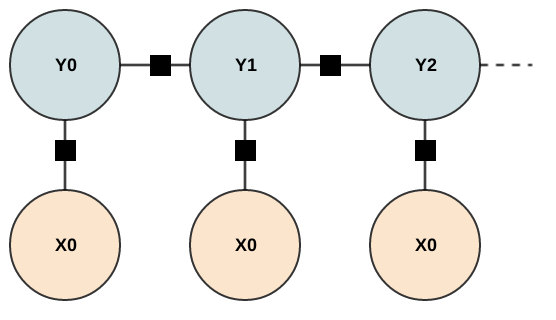
Undirected graph - markov random field
Factors on state transitions and factors on X to Y (sounds like an HMM right? but wait!)
Factors are not probability distributions — they don't have to sum to one
We normalize over the entire sequence, not at each step

### Conditional Random Fields Sorry for the math :( `$$p(\textbf{y} | \textbf{x}) = \frac{1}{Z(\textbf{x})} \prod_{t=1}^{T} \exp \left\lbrace \sum_{k=1}^{K} \theta_k f_k(y_t, y_{t-1}, \textbf{x}) \right\rbrace $$` * The `$\frac{1}{Z(\textbf{x})}$` is normalizing over the whole sequence * Most important part is feature function: `$f_k(y_t, y_{t-1}, \textbf{x})$`

### Conditional Random Fields Feature function `$f_k(y_t, y_{t-1}, \textbf{x})$` * $y_t$ output label at time $t$ * $y_{t-1}$ output label at previous time step * $\textbf{x}$ whole input sequence Can use information from any part of the input sequence for step $t$ - much **more flexible than HMM** CRFs can have _many_ feature functions (millions is not uncommon) **Regularization** and the discriminative aspect of CRFs allow them to effectively deal with sparse features

### Conditional Random Fields POS tagging example feature functions: * Return 1 if this word end in _-ly_ * Return 1 if the _next_ word end in _-ly_ * Return 1 if sequence ends in a '?' * Return 1 if the _next_ word is an _article_ (a, an, etc) * Return 1 if the _prev_ word is a preposition (of, at, to, etc) Provide expert knowledge via feature engineering. Let optimization figure out which parts are important and which aren't.

### Conditional Random Fields Optimization is tractable because the CRF equation is _convex_ and we can use typical gradient + Hessian methods to find optimal parameters in finite time. In practice, million features with ~100,000 training examples takes 3-10 hours on gcloud 32 core instances.

Conditional Random Fields

Comparing performance on address sequence tagging

123 W Main St

ST_NUMBER PRE_DIRECTIONAL STREET DESIGNATOR

	Token Accuracy	Sequence Accuracy
HMM	~90%	~80%
CRF	98.99%	96.67%

Sorry I don't have the precise numbers for the HMM version, and I didn't have time to dig it out of git and re-run

### Conditional Random Fields Problems: * Linear-chain CRFs can only use previous step(s) like HMMs * Given the larger feature space, CRFs degenerate quicker with higher-orders (compared to HMMs) * Still a lot of feature engineering to do * ... wouldn't it be nice if we could automate that...

# Act 3 Recurrent Neural Networks

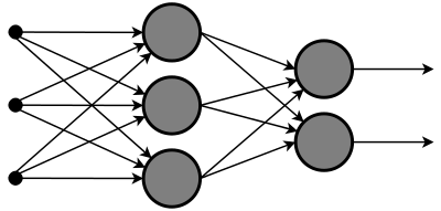
### Deep Learning Deep learning is a huge umbrella term for fancy neural network topologies + lots of tricks to make training robust * Feed Forward Neural Networks for classification, regression * Need some _memory_ to allow previous time steps to influence future time steps ![FF ANN](/talks/ffann-1.png)

Long Short-term Memory Neural Networks

Recurrent neural networks have self-connections that provide such a memory
Consequence of back propagation through many layers: _vanishing_ gradient
Want: a way to remember things across activations (and forgetting is important too)

LSTM Schematic

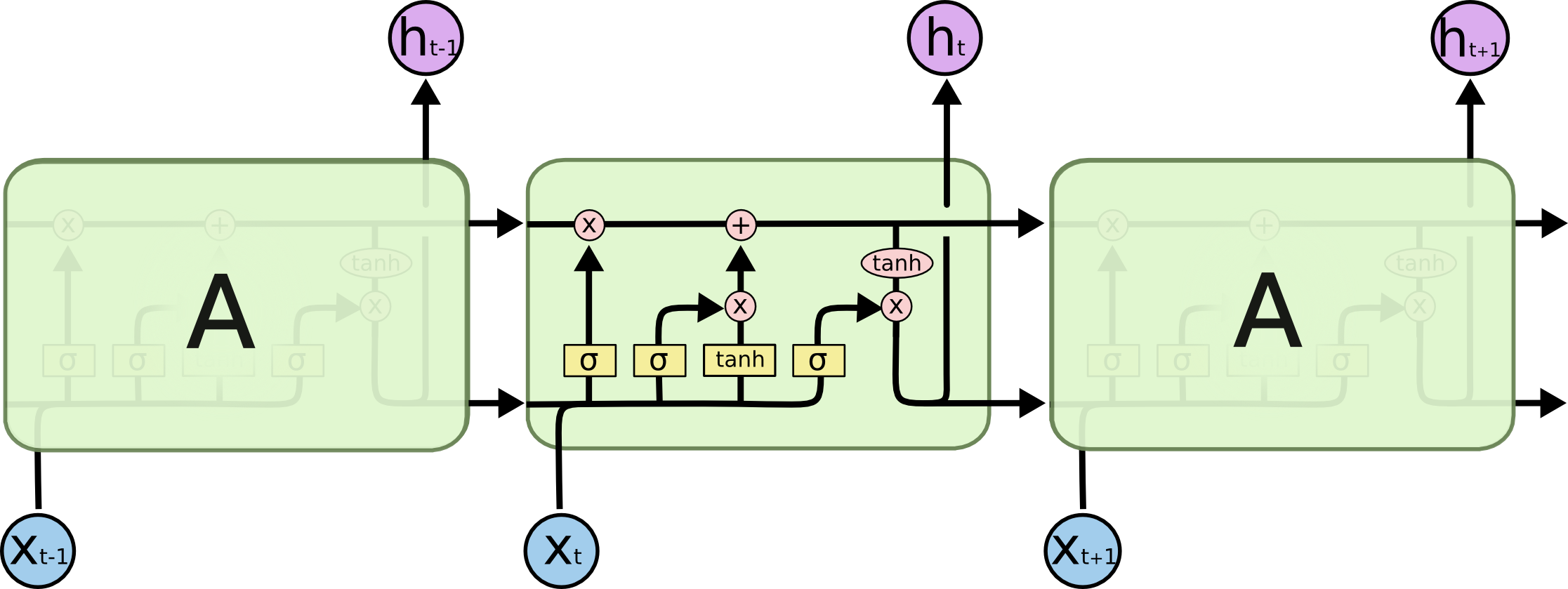
LSTMs

Cell is the internal memory across activations
Gates to control that internal memory
- Forget gate - Should we forget the prev value?
- Input gate - How much should we update our cell?
- Output gate - How much should we output?

LSTM Schematic

Net effect: ability to learn long term memories, gradient doesn't vanish

LSTMs

One example of a performance comparison: Predicting phonemes for words

"discussion" → dɪˈskʌʃən

	Word Accuracy	% Improve
HMM	0.7520
CRF	0.7592	0.96%
LSTM	0.7870	4.65%

### Takeaways * HMMs are _generative_, CRFs are _discriminative_. They model different things with probabilities. * HMMs can be extended to higher orders more easily than CRFs * LSTMs aren't statistical machines at all (for better, for worse) * LSTMs are state-of-the-art for many tasks

### Use **HMMs** when: * Structure in **output** is more important than structure in **input** * use higher order HMMs * You want a probabilistic model * for Bayesian treatments, domain specific regularization, etc. * Simple and fast execution — compared to others * You want to learn a model, then use that to _generate_ sequences

### Use **CRFs** when: * Structure in **input** is more important than structure in **output** * Use lower order chain with rich feature functions * Lots of _information_ in the input side, especially when you want non-local features * You want a probabilistic model * Interpretable probabilities since its conditioned over _entire_ sequence

### Use **LSTMs** when: * State of the art accuracy is the most important concern (not compactness or speed) * You have fast GPUs or a lot of cloud time (training can be pretty long) * You have some experience with deep learning * Toolkits are improving, but still a lot of black magic, rules of thumb * I think its easier to screw up LSTMs than HMMs (could be wrong in near future)

# Questions? * [Andrew Moore's tutorials](http://www.cs.cmu.edu/~awm/tutorials.html) * [Andrew Moore's HMM tutorial](http://www.autonlab.org/tutorials/hmm.html) * [Intro to CRFs](http://blog.echen.me/2012/01/03/introduction-to-conditional-random-fields/) * [Colah's Blog - LSTM Info](http://colah.github.io/posts/2015-08-Understanding-LSTMs)